Do we need central banks?

Monday 29th February, 2016 Ben Duffieldadam smith institute, asi, central bank, NGDP, OMO, sound moneyLeave a comment

I have recently been trying to collect opinions as to why we assume we need central banks (prompted somewhat by the lead-up to the december 2015 rate hike).

I was thus happy to come across The Adam Smith Institute’s Sound Money (published January 2016), which argues that, along with other reforms, we actually should aim for free banking (i.e. no central bank).

Sound Money - Executive Summary

Definitely worth the read, if for no other reason than to challenge the things we take for granted (most responses I get to “why do we even need central banks?” take the form of “because we need a lender of last resort” or that “it would be infeasible to not”).

The arguments for NGDP (nominal GDP) targeting are also compelling.

Firstly, if you have a positive real shock (i.e. productivity rises) this will put downward pressure on prices. Under an inflation target central banks would respond by easing policy, but this could generate asset bubbles. An NGDP target would allow prices to fall to reflect the increased productivity. Indeed according to George Selgin’s “productivity norm” prices should be allowed to fall. Maintaining an inflation target of 2% would not only generate loose monetary conditions but also deprive us of a benign price deflation.

Secondly, if there is a negative real shock (e.g. a natural disaster) then prices should rise, because the price system is supposed to reflect real scarcities. But an inflation-targeting regime would have to respond to the inflationary pressure by tightening policy, and reducing growth.

On Sense and Reference

Wednesday 20th May, 2015Monday 18th May, 2015 Ben Duffieldfrege, reference, senseLeave a comment

A little bit of Frege by someone who probably doesn’t understand.

$a = a$ holds a priori. Kant would say it’s “analytic”.

Using $*$ to denote “the referent of”, expressions of the kind $*a = *b$ , rather than being self-evident, instead contain extension of knowledge. We’ve gained the insight that $a$ and $b$ refer to the same thing: as a silly example, the learning that “the ratio of a circle’s circumference to its diameter” refers to the same thing as “the infinite sum $4 (1 - \frac{1}{3} + \frac{1}{5} - \frac{1}{7} + \ldots )$ “.

We can have $*a = *b$ without it being the case that $a = b$ . The signs are not the same. In what ways do they differ?

Even if the referents are the same, the sense is also important.

Uniqueness?

a referent potentially has many signs.
(we hope) a sign in a given context has at most referent.
It may have none – consider the sign “the celestial body most distant from the earth”.

In natural language normally when we use words (without quotes) we intend to speak of their referent. If we want to refer to the sign itself we can quote the words. We can also call out the sense explicitly. When using natural language we quite often presuppose the existence of a referent.

We can attempt to make some definitions a tad more concrete.

a sense/thought is the way in which a sign refers to an object.
a proper name/sign/word/expression expresses/has a sense and refers to/references/designates its referent.
a referent is an object of some kind.
a sentence is a special kind of expression which has a truth-value as its referent

a truth-value is something which is either true or false, with no other possibilities.

Now, we postulate to the following invariant: the truth-value of a sentence should remain unchanged when we replace a part of the sentence with an expression having the same referent. The truth value of the sentence is in the space of referents and isn’t effected by the sense.
Performing a substitution may well change the sense.

Subtleties here include:

Due to the quirks of natural language, parts of a sentence might be implicitly quoted – the referent of the quoted expression is the sense of the unquoted expression.
Frege enumerates many different grammatical constructs with edge-cases.
A ‘part’ of a sentence may not be a contiguous string of words, so one has to be careful when performing replacements.

Apparently Russell blows a lot of this stuff up, but I’m not there yet.

Capital in the Twenty-First Century, A Free Nation Deep in Debt, Superintelligence – Three Viewpoints

Tuesday 19th May, 2015Monday 18th May, 2015 Ben Duffieldcapital, foom, freedom, government, growth, piketty, superintelligenceLeave a comment

Piketty’s Capital in the Twenty-First Century, MacDonald’s A Free Nation, Deep in Debt and Bostrum’s Superintelligence: Path’s, Dangers, Strategies speak about some similar topics. I wanted to draw some comparisons.

Capital in the Twenty-First Century	A Free Nation, Deep in Debt	Superintelligence
Inequality as an economic inevitability (ceteris paribus).	Democracy as an economic imperative.	Greater-than-human intelligence as an economic inevitability.
Left unchecked, capitalism (and r > g) will lead to extreme inequality. It should be the role of governments to intervene.	Left unchecked, governments can tend to autocracy and tyranny. A free market in government debt can hold governments accountable.
Long-run global growth will never exceed 1.5%		“History, at the largest scale, seems to exhibit a sequence of distinct growth modes, each much more rapid than its predecessor” Pleistocene Society – 224000 year doubling time Farming Society – 909 year doubling time Industrial Society – 6.3 year doubling time
	A large number of citizen bondholders ensures a government enacts the desires of its citizenry.	Seed AI could be given a goal of carrying out humanity’s “coherent extrapolated volition”.
The World Wars had a large impact on the structure of capital – destroying a large amount of capital stock and so increasing labour’s share of income.	The World Wars changed the role of the citizen bondholder. Firstly in the sense of measures such as rationing and compulsory saving. Secondly, the post-war globalisation means “there is nothing patriotic or intrinsically democratic about [today’s bond markets]. Credit markets still generally rank democracies more favourably than other forms of government”.
Without intervention, in the long-run labour’s share of income will decrease. This is inevitable given how return on capital (r) will be larger than growth (g).		After an emergence of superintelligence, “the income share received by labour would then dwindle to practically nil”. All income will be derived from capital, whilst labour income would be driven to the cost of computation. On the other hand, world GDP would undergo extremely rapid expansion. The doubling time could be days, hours or minutes.
Growth from population increases will become less important as world population plateaus and birth rates fall in the developing world. In western europe, population will decrease putting downward pressure on growth (all growth must come from productivity gains).		Simulated minds (mind-uploading) and space colonization implies a potential for extremely rapid population growth. Alternatively, if humans do not end up owning the superintelligence revolution, Malthus rears his ugly head.
We ignore human capital throughout.		Human capital! This is very important. Could also be crucial in keeping emergence of superintelligence in check.
Inequality is BAD.		Inequality may have “been [one of] the greatest humanitarians”. It enabled “average level of well-being to occasionally bob up slightly above that of life at the very margin of subsistence”.

No real synthesis at this point. I think my biggest problem with Piketty is still the assumption of 1.5% cap on growth – Marx + 1.5%.

Death by Watermelon

Monday 18th May, 2015Monday 18th May, 2015 Ben DuffieldLeave a comment

How much watermelon is deadly?

There are many conceivable ways in which a watermelon could in fact prove fatal. One potentially toxic aspect of watermelon is right there in the name – water.

Water, when consumed in large enough quantities, can lead to hyponatremia – “insufficient salt in the blood”. At this point, osmotic pressure makes cells swell up, leading to bad things.

How much is too much? Studies aren’t entirely conclusive. The figure is somewhere around 90ml/kg of body mass. For an average adult human, around 6 litres of water may prove fatal.

For an average adult watermelon, the mass of flesh weighs around 6.3kg. At 92% water by mass, that’s 5.8 litres of water.

Eating a slightly above-average sized watermelon could prove fatal!

This is ignoring a couple of potentially important points:

the figure of 6 litres is for consumption in one go – eating a whole watermelon in one go would be quite a feat
we’re completely ignoring that watermelon isn’t just water. It will actually contain electrolytes. If you salt your watermelon, even better

Be careful.

Changing the Spark Context of an existing RDD

Sunday 15th March, 2015Sunday 15th March, 2015 Ben Duffieldapache spark, cluster, proxy, rdd, spark2 Comments

Spark RDDs are supposed to be Resilient. If something bad happens whilst computing, we can recover! At least, that’s the idea.

scala> val myRdd = sc.parallelize(Seq(1,2,3))
myRdd: org.apache.spark.rdd.RDD[Int] = ParallelCollectionRDD[0] at parallelize at <console>:12
scala> sc.stop

If we stop the spark context for any reason, we now find our RDD is useless!

scala> myRdd.first
java.lang.IllegalStateException: SparkContext has been shutdown
at org.apache.spark.SparkContext.runJob(SparkContext.scala:1316)
at org.apache.spark.SparkContext.runJob(SparkContext.scala:1339)
at org.apache.spark.SparkContext.runJob(SparkContext.scala:1353)
at org.apache.spark.rdd.RDD.take(RDD.scala:1098)

This isn’t good at all! Let’s make a new spark context.

scala> val sc = new org.apache.spark.SparkContext("local[8]", "new context")
sc: org.apache.spark.SparkContext = org.apache.spark.SparkContext@542beecb

We now need to inject this back into our RDD. The spark context is stored in a private field, so we have to reach for reflection.

val rddClass = classOf[org.apache.spark.rdd.RDD[_]]
val scField = rddClass.getDeclaredField("_sc") // spark context stored in _sc
scField.setAccessible(true) // now we can access it

Now we just set the spark context.

scField.set(myRdd, sc)

Observe that this works!

scala> myRdd.sum
res5: Double = 6.0
scala> myRdd.first
res6: Int = 1

This is quite scary and probably should not be used for anything real. Additionally we had an RDD with many dependencies, we’d have to crawl the the dependencies and swap it out in every place (I think).

Another approach might be to instead produce a dynamic proxy for the spark context which allows you to point at some true spark context, and then just swap it out there.

What are we actually trying to do here? If we have a long-running application which allows users to create RDDs, it would be nice to be able to recover from spark cluster bounces. We could keep track of the operations required to produce the RDDs in the first place (which is arguably a better approach) but I decided to spend thirty minutes poking around anyway, and was pleasantly surprised at the (illusion of) progress I made!

Cosine Similarity, Pearson Correlation, Inner Products

Thursday 14th August, 2014Thursday 14th August, 2014 Ben Duffieldcorrelation, cosine similarity, dot product, haskell, inner product, pearson correlation, similarityLeave a comment

To begin, a criticism

I picked up the Haskell Data Analysis Cookbook. The book presents examples of comparing data using Pearson Coefficient and using Cosine Similarity.

pearson xs ys = (n * sxy - sx * sy) / sqrt ((n * sxx - sx * sx) * (n * syy - sy * sy))
   where
      n = fromIntegral (length xs)
      sx = sum xs
      sy = sum ys
      sxx = sum $ zipWith (*) xs ys
      syy = sum $ zipWith (*) ys ys
      sxy = sum $ zipWith (*) xs ys

cosine xs ys = dot d1 d2 / (len d1 * len d2)
   where
      dot a b = sum $ zipWith (*) a b
      len a = sqrt $ dot a a

Although these code snippets are both calculating the ‘similarity’ between two vectors and actually, as we shall see, share a lot of structure, this is not at all apparent from a glance.

We can fix that however…

Definition of an Inner Product

An inner product is conceptually a way to see how long a vector is after projecting it along another (inside some space).

Formally, an inner product is a binary operator satisfying the following properties

Linearity

$\langle u+v,w \rangle = \langle u,w\rangle + \langle v,w\rangle$
$\langle \alpha u,w\rangle = \alpha\langle u,w\rangle$ for $\alpha \in \mathbb{R}$
We are saying that we can push sums inside on the left to being outside. We can also push out constant factors.

(Conjugate) Symmetry

$\langle u,v \rangle = \langle v,u \rangle$ or in the complex case, $\langle u,v \rangle = \overline{\langle v,u \rangle}$
In the real case, we’re saying everything is symmetric – it doesn’t matter which way you do it. In the complex case we have to reflect things by taking the conjugate.

Positive Definiteness

$\langle u,u \rangle \ge 0$ with equality iff $u = 0$
Here we’re saying projecting a vector onto itself always results in a positive length. Secondly, the only way we can end up with a result of zero is if the vector itself is of length 0.

From Inner Product to a notion of ‘length’

Intuitively a distance between two things must be

positive or zero (a negative distance makes not too much sense), with a length of zero corresponding to the zero vector
linear (if we scale the vector threefold, the length should also increase threefold)

Given that $\langle u,u \rangle \ge 0$ we might be tempted to set $length(a) := \langle u,u \rangle$ but then upon scaling $u \rightarrow \alpha u$ we get $length(\alpha u) := \langle \alpha u, \alpha u \rangle = \alpha^2 \langle u,u \rangle$ – we’re not scaling linearly.

Instead defining $||a|| := \sqrt{\langle a,b \rangle}$ everything is good!

Similarity

Now, in the abstract, how similar are two vectors?

How about we first stop caring about how long they are, and want them just to point in the same direction. We can project one along the other and see how much it changes in length (shrinks).

Projecting is kind of like seeing what its component is in that direction – i.e. considering 2-dimensional vectors in the plane, projecting a vector onto a unit vector in the $x$ direction will tell you the $x$ component of that vector.

Let’s call two vectors $a$ and $b$ .

Firstly let’s scale them to be both of unit length, $\hat{a} = \frac{a}{||a||}, \hat{b} = \frac{b}{||b||}$

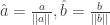
Now, project one onto the other (remember we’re not caring about order because of symmetry).
$similarity(a,b) := \langle \frac{a}{||a||}, \frac{b}{||b||} \rangle$

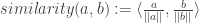
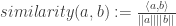
Using linearity we can pull some stuff out (and also assuming everything’s happily a real vector – not caring about taking conjugates)…
$similarity(a,b) := \frac{\langle a, b \rangle}{||a|| ||b||}$

Making Everything Concrete

Euclidean Inner Product

The dot product we know and love.
$a \dot b = a_1 b_1 + \dots + a_n b_n$

Plugging that into the similarity formula, we end up with the cosine similarity we started with!

Covariance Inner Product

The covariance between two vectors is defined as $Cov(X,Y) = \mathbb{E}((X - \mathbb{E}(X))(Y - \mathbb{E}(Y)))$ where we’re abusing the notion of expectation somewhat. This in fact works if X and Y are arbitrary L2 random variables… but for the very concrete case of finite vectors we could consider $\mathbb{E}(X) = \frac{1}{n}(x_1 + \dots + x_n)$ .

We’ve said in our space, to project a first vector onto a second we see how covariant the first is with the second – if they move together or not.

Plugging this inner product into the similarity formula, we instead get the pearson coefficient!

In fact, given $Cov(X,X) = Variance(X)$ , in this space we have $length(X) = \sqrt{Variance(X)} = StdDev(X) =: \sigma_X$ ,

i.e. $similarity(X,Y) = \frac{Cov(X,Y)}{\sigma_X \sigma_Y}$ .

Improving the code

Now that we know this structure exists, I posit the following as being better

similarity ip xs ys = (ip xs ys) / ( (len xs) * (len ys) )
   where len xs = sqrt(ip xs xs)

-- the inner products
dot xs ys = sum $ zipWith (*) xs ys

covariance xs ys = exy - (ex * ey)
   where e xs = sum xs / (fromIntegral $ length xs)
         exy = e $ zipWith (*) xs ys
         ex = e xs
         ey = e ys

-- the similarity functions
cosineSimilarity = similarity dot
pearsonSimilarity = similarity covariance

Things I’m yet to think about

…though maybe the answers are apparent.

We have a whole load of inner products available to us. What does it mean to use those inner products?
E.g. $\langle f,g \rangle = \int^{-\pi}_{\pi} f(t) \overline{g(t)} \, \mathrm{d}t$ on $\mathbb{L}^2[-\pi,\pi]$ – the inner product producing the Fourier transform. I’m not the resulting similarity is anything particularly special though…

Notes: First Steps with the Interactive Brokers API (OS X Mavericks)

Sunday 15th June, 2014Sunday 15th June, 2014 Ben DuffieldIB, interactive brokers, java, mac os xLeave a comment

Setup

IB Workstation

In order to use the API the IB Workstation must be installed and running – one then connects to this using the API. Installation is available for Mac, Linux and Windows – for mac the automatic pkg is here.

IB API

Next step is to download the API – a collection of java source files which handle talking to the IB Workstation. Download the jar and extract it somewhere.

IB Controller

Manually running the GUI app each time/manually clicking through dialogs etc, is a pain. To mitigate this the IB Controller github project provides a wrapper around launching/controlling the app. Getting this working was just a matter of following the userguide.

Creating a Simple Automated Client (Eclipse)

Ultimately this’ll be done with gradle, but for now let’s just quickly use eclipse.

Create a new eclipse project
Add the folder ‘javaclient’ from wherever the API was extracted as a linked source folder (right click on project -> build path -> link source folder)
We’ll use classes in com.ib.controller
- instantiate an ApiController
- instantiate a NewContract
- instantiate a NewOrder
- call the controller’s placeOrModifyOrder method (for now just use a no-op IOrderHandler)

Next Steps

I feel it’s important for this type of thing (i.e. time sensitive, immediate monetary penalties for errors) to focus on verification/programming defensively.

Thinking in pseudocode I feel like I want to place an order, and be notified if it’s not filled in $timeout seconds/any other error happens. I also feel like I want to maintain a local version of the truth, and always compare this against what the API reports as the truth before doing anything.

List of Datasets, List of Lists of Datasets

Sunday 1st June, 2014 Ben Duffielddata, dataset, lending club, medical datasets, opendata, whoLeave a comment

Consider this sort of a public-facing list of datasets I’ve found interesting, have played with or want to play with.

List of Datasets

Lending Club

Peer to peer credit marketplace Lending Club publishes data on issued and declined loans. https://www.lendingclub.com/info/download-data.action

World Health Organisation

The WHO publishes many interesting datasets at http://www.who.int/research/en/. They don’t however do a great job of linking to the raw datasets: http://www.who.int/healthinfo/statistics/mortality_rawdata/en/ is a comprehensive dataset providing mortality rates for all reporting countries, but difficult to find from the navigation.

New York Times

The New York Times has a fairly comprehensive open api, documented at http://developer.nytimes.com/docs

Divvybikes

The Chicago public cycle hire scheme (akin to New York’s Citibike, London’s ~~Barclays~~ Boris Bike) published data on 750 000 trips made for their data challenge. http://divvybikes.com/datachallenge

Outpan

Outpan aims to provide a single database for turning barcodes into product information. Not extremely complete. http://www.outpan.com/index.php

Medicare

Under the efforts of transparency, a dataset containing information around usage of Medicare. Could make a complement to some of the other medical datasets available. http://www.cms.gov/Research-Statistics-Data-and-Systems/Statistics-Trends-and-Reports/Medicare-Provider-Charge-Data/Physician-and-Other-Supplier.html

List of Lists of Datasets

http://rs.io/2014/05/29/list-of-data-sets.html – 100+ Interesting Data Sets for Statistics. Pretty much all of these are really great!

Looking for interesting data sets? Here’s a list of more than 100 of the best stuff, from dolphin relationships to political campaign donations to death row prisoners.
http://bagrow.com/dsv/datasets.html – contains links some datasets and some lists of datasets. Perhaps this should come under the section lists of lists of lists of datasets.
https://en.wikipedia.org/wiki/Open_data
http://www.quora.com/Where-can-I-find-large-datasets-open-to-the-public

How Spark does Class Loading

Sunday 30th March, 2014 Ben DuffieldClass Server, classloading, java, jetty, jvm, remote, scala, server, sparkLeave a comment

Using the spark shell, one can define classes on-the-fly and then use these classes in your distributed computation.

Contrived Example

scala> class Vector2D(val x: Double, val y: Double) extends Serializable {
| def length = Math.sqrt(x*x + y*y)
| }
defined class Vector2D
scala> val sourceRDD = sc.parallelize(Seq((3,4), (5,12), (8,15), (7,24)))
sourceRDD: org.apache.spark.rdd.RDD[(Int, Int)] = ParallelCollectionRDD[5] at parallelize at :13
scala> sourceRDD.map(x => new Vector2D(x._1, x._2)).map(_.length).collect()
14/03/30 09:21:59 INFO SparkContext: Starting job: collect at :17
...snip...
res1: Array[Double] = Array(5.0, 13.0, 17.0, 25.0)

In order for the remote executors here to actually run your code, they must have knowledge of the Vector2D class, yet they’re running on a different JVM (and probably different physical machine). How do they get it?

we choose a directory on disk to store the class files
a virtual directory is created at SparkIMain:101
a scala compiler is instantiated with this directory as the output directory at SparkIMain:299
this means that whenever a class is defined in the REPL, the class file is written to disk
a http server is created to serve the contents of this directory at SparkIMain:102

we can see info about the Http server in the logs:

14/03/23 23:39:21 INFO HttpFileServer: HTTP File server directory is /var/folders/8t/bc2vylk13j14j13cccpv9r6r0000gn/T/spark-1c7fbed7-5c87-4c2c-89e8-be95c2c7ac54
14/03/23 23:39:21 INFO Executor: Using REPL class URI: http://192.168.1.83:61626

the http server url is stored in the Spark Config, which is shipped out to the executors
the executors install a URL Classloader, pointing at the Http Class Server at Executor:74

For the curious, we can figure out what the url of a particular class is and then go check it out in a browser/with curl.

def urlOf[T:ClassTag] = {
   val clazz = implicitly[ClassTag[T]].erasure
   Seq(sc.getConf.get("spark.repl.class.uri"),
       clazz.getPackage.getName,
       clazz.getName).mkString("/")
}

Do it yourself

It’s pretty trivial to replicate this ourselves – in Spark’s case we have a scala compiler which writes the files to disk, but assuming we want to serve classes from a fairly normal JVM with a fairly standard classloader, we don’t even need to bother with the to disk. We can grab the class file using getResourceAsStream. It also doesn’t require any magic of scala – an example class server in java using Jetty:

class ClasspathClassServer {
	private Server server = null;
	private int port = -1;

	void start() throws Exception {
		System.out.println("Starting server...");
		if(server != null) {
			return;
		}

		server = new Server();
		NetworkTrafficSelectChannelConnector connector = new NetworkTrafficSelectChannelConnector(server);
		connector.setPort(0);
		server.addConnector(connector);

		ClasspathResourceHandler classpath = new ClasspathResourceHandler();

		server.setHandler(classpath);
		server.start();

		port = connector.getLocalPort();
		System.out.println("Running on port " + port);
	}

	class ClasspathResourceHandler extends AbstractHandler {
		@Override
		public void handle(String target, Request baseRequest, HttpServletRequest request, HttpServletResponse response)
					throws IOException, ServletException {
			System.out.println("Serving target: " + target);

			try {
				Class<?> clazz = Class.forName(target.substring(1));
				InputStream classStream = clazz.getResourceAsStream('/' + clazz.getName().replace('.', '/') + ".class");

				response.setContentType("text/html;charset=utf-8");
				response.setStatus(HttpServletResponse.SC_OK);
				baseRequest.setHandled(true);

				OutputStream os = response.getOutputStream();

				IOUtils.copy(classStream, os);
			} catch(Exception e) {
				System.out.println("Exception: " + e.getMessage());
				baseRequest.setHandled(false);
			}
		}
	}
}

It’s then just a matter of setting up a URL Classloader on the other side!

Further Examples

http://quoiquilensoit.blogspot.com/2008/02/generic-compute-server-in-scala-with.html: An example of using a similar technique to write a ‘compute server’ in scala – somewhat akin to a very stripped down version of Spark.

Chunkify – Grouping series in pandas for easy display

Wednesday 5th March, 2014Monday 3rd March, 2014 Ben Duffieldchunk, dataframe, ipython, notebook, pandas, population data, python, whoLeave a comment

Continuing with the same population data-set from last time, say we wanted to group countries by when their last valid entry in the population data table.

last_year_of_data = pop_stats.groupby('Name')['Year'].max().reset_index()
last_year_of_data.head()

	Name	Year
0	Albania	2004
1	Antigua and Barbuda	1983
2	Argentina	1996
3	Armenia	2012
4	Australia	2011

Let’s say we want to display these groups of countries in chunks – enter chunkify.

def chunkify(series, into=4):
    #ensure the series has a sequential index
    series = series.reset_index(drop=True)
    #chunk the series into columns
    columns = [series[range(i, series.size, into)]
                        .dropna()
                        .reset_index(drop=True)
                    for i in range(into)]
    #stick the columns together
    df = pd.concat(columns, axis=1)
    #rename the columns sequentially
    df.columns = range(into)
    return df

Usage is simple.

last_year_of_data.groupby('Year')['Name'].apply(lambda x : chunkify(x, 3))\
    .fillna('')

Voilà!

(truncated…)

		0	1	2
Year
2008	0	Malaysia	Maldives
2009	0	Fiji	Iceland	Ireland
2009	1	Jordan	New Zealand	South Africa
2010	0	Bahrain	Belarus	France
	1	Georgia	Italy	Kazakhstan
	2	Kyrgyzstan	Lithuania	Mongolia
	3	Romania	Russian Federation	Slovakia
	4	Slovenia	Sweden	Switzerland
	5	TFYR Macedonia	United Kingdom	United Kingdom, Northern Ireland
2011	0	Australia	Bosnia and Herzegovina	Brunei Darussalam
	1	Bulgaria	Cyprus	Denmark
	2	Egypt	Finland	Greece
	3	Hong Kong SAR	Japan	Kuwait
	4	Malta	Mauritius	Netherlands
	5	Poland	Portugal	Qatar
	6	Republic of Korea	Rodrigues	Singapore
	7	Spain	United Kingdom, Scotland
2012	0	Armenia	Austria	Belgium
	1	Croatia	Czech Republic	Estonia
	2	Germany	Hungary	Israel
	3	Latvia	Luxembourg	Norway
	4	Republic of Moldova	Serbia	Seychelles
	5	Ukraine	United Kingdom, England and Wales

Share this:

Uniqueness?

Share this:

Share this:

Share this:

Share this:

To begin, a criticism

Definition of an Inner Product

Linearity

(Conjugate) Symmetry

Positive Definiteness

From Inner Product to a notion of ‘length’

Similarity

Making Everything Concrete

Euclidean Inner Product

Covariance Inner Product

Improving the code

Things I’m yet to think about

Share this:

Setup

IB Workstation

IB API

IB Controller

Creating a Simple Automated Client (Eclipse)

Next Steps

Share this:

List of Datasets

Lending Club

World Health Organisation

New York Times

Divvybikes

Outpan

Medicare

List of Lists of Datasets

Share this:

Contrived Example

Do it yourself

Further Examples

Share this:

Share this: